This tutorial will show you how to plot a possible storm track extending out from a storm center on RADAR. This tutorial will show you how to do this using two different methods. The first (more complicated) method requires the use of traj.gs and information of a future time steps. The 2nd (simpler method) does not require traj.gs, and it only requires information from the current time step.
For both parts of this tutorial, we will use data from the WRF model, as this model outputs both storm motion vectors and RADAR reflectivity. So, without further delay, lets get started with the 1st method.
Plotting Storm Tracks - Method 1:
As stated, this method is a bit more complicated and requires more effort. That being said, you can plot more detailed storm tracks using this method over the 2nd. Before we get started there is one
major caveat regarding this method. Usually, when I write up tutorials I have you access data online through the NOMADS server (by use of the '
sdfopen' command). Unfortunately, the
traj.gs script requires you have a .ctl file, so accessing the data online through the
'sdfopen' command is not going to work. Additionally, while it is possible to modify the traj.gs function to be compatible with the netcdf data, plotting trajectories using online data will take a really, really, really long time. What I have done, is included a small sample of WRF model data from July 17th 2013, including a .ctl file for you to use as an example. So unless you have your own model data that includes information regarding storm track and reflectivity, it is recommended you use the data provided here.
Required for method 1:
Now that you have the required files and data, I will briefly describe what we are going to do, and show you the result. Basically, all we do is plot reflectivity and then use the
mfhilo function to find local maxima in reflectivity and use traj.gs to plot forward trajectories. The following image serves as an example.
 |
| Example of plotted Storm tracks from WRF model using the 1st method |
|
|
|
|
Now, the first thing we will need to do is open the file, and set our basic parameters.
'open ARW_20120717.ctl'
'clear'
'set mpdset hires'
'set parea 0.5 10.0 0.5 7.5'
At this point we are going to deviate from our main script and open up traj.gs. It is important to open traj.gs because we need to make a few edits in the code. First of all, we need to change what traj.gs reads as its "U" and "V" components. To do this you need not look further than line 18 in traj.gs. Here you can set what model variables _U and _V point to. Since we want storm track, storm motion seems an appropriate variable to me. So first we need to change the following pieces of code
from:
_U='U'
_V='V'
to:
_U='ustm6000_0m'
_V='vstm6000_0m'
Once this is done, we need to make a couple more small edits before we return to the main script (I should note here that it might be wise to save a special version of traj.gs just for this use).
Basically, we are really only interested in the forward trajectory, so we need to change the threshold used in the while loop that has the variable volta from 2 to 1 (line 40). This basically only allows the plotting of the forward trajectories instead of both forward and back.
The last small edit that we need to make is on line 46, the one that sets the variable "TM." Unless you want to plot out the possible trajectory for the ALL time steps (for the sample data here that is 48 hours) you want to change this variable. I figure 5 hours (or 5 time steps) is long enough, for a trajectory, so I changed this variable to _Tini+5, or the current time + 5 time steps into the future.
So, that does it for our edits to traj.gs and we are now ready to write out the rest of the script.
For this example, we will choose the 4th time step, so we start by declaring our domain and plotting our variable, if you have colorset.gs you can pick one of the reflectivity color scales, or if not you can set it manually yourself. This tutorial will use the "Wunder1" option from colorset.gs
'set t '4
'set lat 38 49'
'set lon -80 -65'
'set gxout shaded'
'colorset Wunder1'
'd refcclm'
'cbar' ;*
Its assumed you have cbar.gs, if not you shouldn't be reading advanced tutorials.
Now your variable is plotted and we need to find the local maxima of reflectivity. For this we use the mfhilo function (similar to the
tutorial on SLP maps). However, this time we are only interested in the maxima. Below is the loop used to find reflectivity maxima, and plot trajectories.
radius=25
cint=15
'mfhilo refcclm CL h 'radius', 'cint
ref_data=result
i=3
minmax = sublin(result,i)
check=subwrd(minmax,1)
while(check = 'H')
use_lat = subwrd(minmax, 2)
use_lon = subwrd(minmax, 3)
mag=subwrd(minmax,5)
if(mag > 35)
'q w2xy 'use_lon' 'use_lat
x_min = subwrd(result,3)
y_min = subwrd(result,6)
'set line 0'
'draw mark 3 'x_min' 'y_min' 0.15'
'traj 'use_lon' 'use_lat
endif
i=i+1
minmax = sublin(ref_data,i)
check=subwrd(minmax,1)
endwhile
Lets break down this loop a little bit. So, basically you use the mfhilo function to generate a list of maxima in reflectivity. Then you loop through each data point, save the lat/lon coordinates (using the
subwrd() function), and then check the reflectivity value against some threshold value that you pick (in this example: 35dBZ). If the reflectivity maximum is greater than this value, you run
traj.gs which plots the forward trajectory, if it does not mean this value, than you move on to the next one.
That's all there is too it, you are done with the first method! Now, you will need to tweak values such as the radius and the contour interval used in the mfhilo function to best fit your requirements, the ones I used in this example provide reasonable results, but you can (and should) experiment with those.
Now that we have covered the first method, lets start up with the 2nd method.
Plotting Storm Tracks - Method 2:
This method is a little less involved than the first method, and does not require the use of
traj.gs, nor does it require the use of a .ctl file. So for this part of the tutorial, we will simply use the
'sdfopen' command to grab the required data. Again, it is recommended you use
colorset.gs to help you set up color scales. Also, unlike the first method you only require the current time step to plot storm tracks.
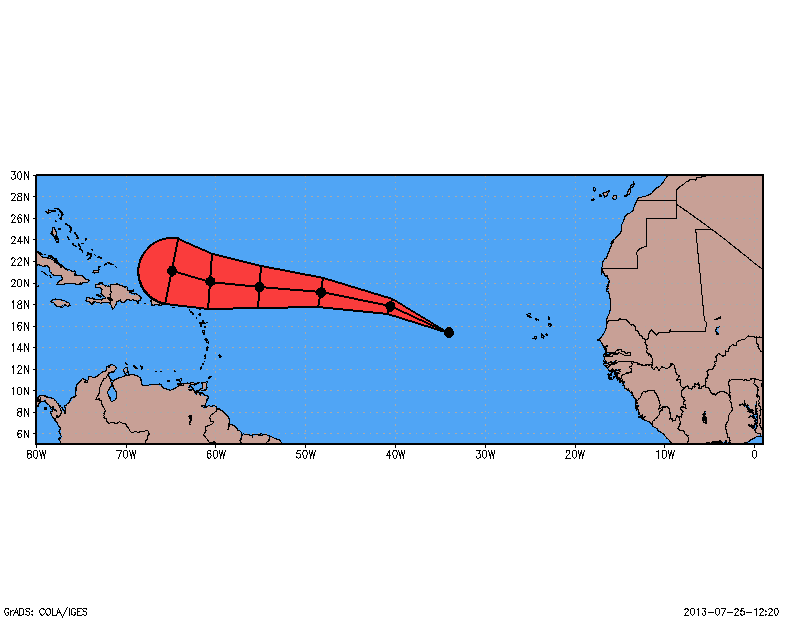
Similar to the first method, we will use the mfhilo function to find local maxima in the reflectivity field. Once a maximum is located, instead of using traj.gs to plot forward trajectories, we will simply take the storm motion at the current time and location, and extrapolate out (in this example 5 hours) from it. The result is a linear storm track, rather than one that includes curves and bends (image shown below).
 |
| Example of plotted storm tracks from the WRF model, using method 2 |
This image is the same time step used in the first method, and as you can see it doesn't look all that dissimilar from the image above. However, you do see the loss in curvature in the storm tracks, which is really all you lose when using this method over the 1st method.
In order to writing time, I am going to gloss over this part here, it is more as it is more thoroughly described in the method 1 section. All I am doing though is opening the file and plotting the variable.
'sdopen http://nomads.ncep.noaa.gov:9090/dods/hiresw/hiresw20130717/hiresw_eastarw_00z'
'clear'
'set mpdset hires'
'set parea 0.5 10.0 0.5 7.5'
'set t '4
'set lat 38 49'
'set lon -80 -65'
'set gxout shaded'
'colorset Wunder1'
'd refcclm'
'cbar' ;*
Its assumed you have cbar.gs, if not you shouldn't be reading advanced tutorials.
Now, we can get to the bulk of the script. Again, we are going to use the mfhilo function to find the maxima in the reflectivity field.
radius=25
cint=15
'mfhilo refcclm CL h 'radius', 'cint
ref_data=result
i=3
minmax = sublin(result,i)
check=subwrd(minmax,1)
Now things start to differ from the first method. What we need to do is basically place a block of code within the loop that loops through each maximum that converts the storm motion into a change in distance (by multiplying it by time/per timestep - 3600 seconds) and then convert the distance into a change in geographic (lat/lon) coordinates. From there, we just draw marks and lines connecting the dots. The code below shows this process.
_At=6371229
_PI=3.141592654
_D2R=_PI/180
_R2D=180/_PI
if(mag > 35)
'q w2xy 'use_lon' 'use_lat
x_min = subwrd(result,3)
y_min = subwrd(result,6)
'set line 0'
'draw mark 3 'x_min' 'y_min' 0.15'
'set lat 'use_lat
'set lon 'use_lon
'set gxout print'
'd ustm6000_0m'
ustm=sublin(result,2);ustm=subwrd(ustm,1)
'd vstm6000_0m'
vstm=sublin(result,2);vstm=subwrd(vstm,1)
dx_pert=ustm*3600
dy_pert=vstm*3600
time=t
while(time<=max_time)
if(time>t)
xmin=x
ymin=y
endif
'q w2xy 'use_lon' 'use_lat
x = subwrd(result,3)
y = subwrd(result,6)
'set line 2'
if(x>subwrd(xs,1) & x < subwrd(xs,2) & y > subwrd(ys,1) & y < subwrd(ys,2))
'draw mark 3 'x' 'y' 0.075'
endif
if(time>t)
if(x>subwrd(xs,1) & x < subwrd(xs,2) & y > subwrd(ys,1) & y < subwrd(ys,2))
'draw line 'xmin' 'ymin' 'x' 'y
endif
endif
use_lon=use_lon+dx_pert/(_D2R*_At*math_cos(use_lat*_D2R))
use_lat=use_lat+dy_pert/(_D2R*_At)
time=time+1
endwhile
endif
This code represents what you do if your reflectivity value at a given point reaches the minimum threshold required to plot a storm track. The first thing that you do is set the latitude/longitude to the point of interest. Then using the 'set gxout print' command, you grab the U and V storm motion vectors. Once you do this, you calculate the dx/dy per time step variables (dx_pert/dy_pert) by multiplying the storm motion by the seconds/time step. This represents basically the distance you would travel in x/y at this speed in one time step. Now that you have this information, things become pretty simple. You merely draw a mark at the current location using the 'q w2xy' command to convert lat/lon coordinates to page coordinates. Then, you calculate the "future" lat/lon coordinate pair by using the dx_pert/dy_pert and some global geometry to convert physical distance to changes in latitude and longitude. A couple of conditional statements in there help you regulate when to draw lines/marks. It is also important that you ensure the page coordinates of your location fall within your plot area, or you will have lines exceeding your plot boundaries and interfering with your titles and color bars and such. So, putting all of this code together, you get something that looks like this!
radius=25
cint=15
'mfhilo refcclm CL h 'radius', 'cint
ref_data=result
i=3
minmax = sublin(result,i)
check=subwrd(minmax,1)
while(check = 'H')
use_lat = subwrd(minmax, 2)
use_lon = subwrd(minmax, 3)
mag=subwrd(minmax,5)
_At=6371229
_PI=3.141592654
_D2R=_PI/180
_R2D=180/_PI
if(mag > 35)
'q w2xy 'use_lon' 'use_lat
x_min = subwrd(result,3)
y_min = subwrd(result,6)
'set line 0'
'draw mark 3 'x_min' 'y_min' 0.15'
'set lat 'use_lat
'set lon 'use_lon
'set gxout print'
'd ustm6000_0m'
ustm=sublin(result,2);ustm=subwrd(ustm,1)
'd vstm6000_0m'
vstm=sublin(result,2);vstm=subwrd(vstm,1)
dx_pert=ustm*3600
dy_pert=vstm*3600
time=t
while(time<=max_time)
if(time>t)
xmin=x
ymin=y
endif
'q w2xy 'use_lon' 'use_lat
x = subwrd(result,3)
y = subwrd(result,6)
'set line 2'
if(x>subwrd(xs,1) & x < subwrd(xs,2) & y > subwrd(ys,1) & y < subwrd(ys,2))
'draw mark 3 'x' 'y' 0.075'
endif
if(time>t)
if(x>subwrd(xs,1) & x < subwrd(xs,2) & y > subwrd(ys,1) & y < subwrd(ys,2))
'draw line 'xmin' 'ymin' 'x' 'y
endif
endif
use_lon=use_lon+dx_pert/(_D2R*_At*math_cos(use_lat*_D2R))
use_lat=use_lat+dy_pert/(_D2R*_At)
time=time+1
endwhile
endif
i=i+1
minmax = sublin(light_plot,i)
check=subwrd(minmax,1)
endwhile
So, that about wraps it up for this tutorial, a few basic notes are listed below, followed by a downloadable example script.
Notes to remember:
- The 2nd method is a little more versatile as you do not need information about future time
- More applicable to current RADAR data as long as you know the wind components
- Pretty accurate especially for short distances and small timesteps
- You don't have to use "Storm Motion", 850hPa wind vectors probably work similarly
- This goes for both methods
- Doesn't have to be used for RADAR, that's just the example used here.
- You can of course get more fancy with this, change colors, add arrows, etc.
I hope you enjoyed this tutorial, and hopefully you find it useful!
Download Example Script Here